Fish Schooling Density Calculator
Estimate adjusted school count, volumetric density, horizontal density, and average spacing from sonar, drone, cast-net, or visual survey observations.
🏷Schooling labels
📌Schooling presets
⚙School dimensions and survey inputs
Portion of the school core actually sampled by sonar cone, camera frame, or net.
Schooling density estimate
Calculation breakdown
📊Density factor grid
Method correction
Shape volume factor
Packing behavior
Output scale
📘Schooling reference tables
| Species group | Typical length | Loose school | Normal school | Tight school |
|---|---|---|---|---|
| Threadfin or small shad | 2.5-5 in / 6-13 cm | <2 fish per 1k ft³ | 2-12 fish per 1k ft³ | 12+ fish per 1k ft³ |
| Herring or alewife | 4-8 in / 10-20 cm | <1.5 fish per 1k ft³ | 1.5-8 fish per 1k ft³ | 8+ fish per 1k ft³ |
| Sardine or bay anchovy | 2-7 in / 5-18 cm | <4 fish per 1k ft³ | 4-25 fish per 1k ft³ | 25+ fish per 1k ft³ |
| Minnows and shiners | 1.5-4 in / 4-10 cm | <8 fish per 1k ft³ | 8-45 fish per 1k ft³ | 45+ fish per 1k ft³ |
| Young perch or panfish | 2-6 in / 5-15 cm | <1 fish per 1k ft³ | 1-6 fish per 1k ft³ | 6+ fish per 1k ft³ |
| Observation method | Best density use | Count correction | Dimension strength | Watch item |
|---|---|---|---|---|
| 2D sonar arch count | Vertical school slices | +10% | Depth is strong | Cone width changes with depth |
| Side-scan sonar | Footprint and edge length | +6% | Length and width are strong | Shadow overlap can merge fish |
| Forward-facing sonar | Live school tracking | +4% | Range and thickness are good | Ping angle clips the school edge |
| Drone overhead frame | Shallow clear-water schools | -4% | Footprint is strong | Depth estimate needs support |
| Visual bank or boat count | Small visible schools | +18% | Length is fair | Fish under glare are missed |
| Cast-net subsample | Dense bait on flats | +24% | Area is localized | Net avoidance changes counts |
| Shape profile | Volume model | Footprint model | Density meaning | Common setting |
|---|---|---|---|---|
| Oval cruising school | 0.52 x L x W x D | 0.78 x L x W | Balanced spacing | Coves and creek arms |
| Tight bait ball | 0.70 x L x W x D | 0.88 x L x W | Predator-compressed | Offshore chase scene |
| Long ribbon or lane | 0.42 x L x W x D | 0.65 x L x W | Travel corridor | Current seams or flats |
| Diffuse cloud | 0.62 x L x W x D | 0.92 x L x W | Loose aggregation | Open basin forage |
| Vertical screen | 0.58 x L x W x D | 0.54 x L x W | Layered depth band | Smelt or herring at night |
| Patchy edge group | 0.48 x L x W x D | 0.70 x L x W | Broken school edge | Weedline panfish |
| Result check | Low signal | Moderate signal | High signal | Field interpretation |
|---|---|---|---|---|
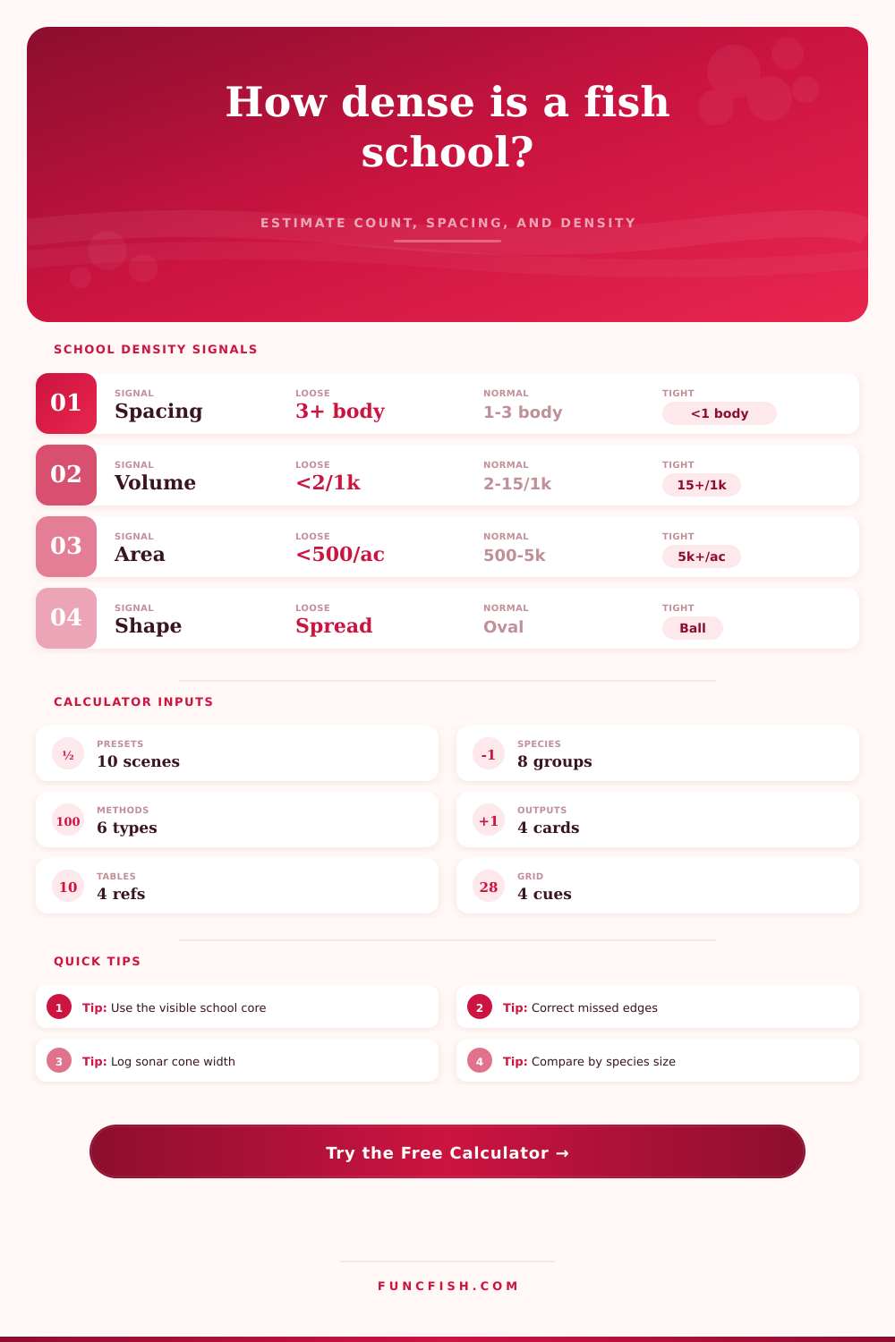
| Volumetric density | <2 per 1k ft³ | 2-15 per 1k ft³ | 15+ per 1k ft³ | Shows how packed the water column is |
| Horizontal density | <500 per acre | 500-5,000 per acre | 5,000+ per acre | Useful for surface frame comparisons |
| Spacing index | 3+ body lengths | 1-3 body lengths | <1 body length | Normalizes density by fish size |
| Correction multiplier | <1.15x | 1.15-1.75x | 1.75x+ | High values mean more survey uncertainty |
💡Density calculation tips
Core boundary: Measure the school core, not the longest stray fish trail. A single distant edge mark can inflate volume and make density look falsely low.
Survey repeat: Recalculate after changing only coverage or edge loss. If the density class flips, treat the estimate as a range rather than a single value.
You know what they say: if you see a bunch of them on your sonar, like a big wiggly blob or just a solid black band across your graph, it’s pay dirt. Then you pull that net up and wonder what happened to all those fish. Where’d they go? The truth is the fish were probably right there. But you overestimated density. There was a school there, but more than likely, you didn’t realize just how vacant it was.
Estimating fish school size by eye are risky business: We cannot accurately determine 3D volume based off 2D surface area. Shallow, sparse clouds of shad may appear as thousands, whereas tight balls of herring could contain more fish different than a diffuse cloud that spans half an acre. A wide, flat ribbon of shad may look like thousands of fish, yet its shallow depth may only contain a few inches of actual fish mass.
How to Measure Fish Density Correctly
The calculator translate raw measurements into adjusted estimates, though knowing how those numbers change will transform guessing into strategizing. But people’s most frequent error is measuring the edge rather than the middle (the core). School boundaries is not crisp lines; they are fuzzy. Fish will break away and wander off in margins. When you stretch your measurement from one extreme mark to another, you expand the volume so much that density appear artificially low.
Density = count/volume. So if you blow up denominator then the density seems too low. You think the water is empty even though it is really full, but distributed. The key is knowing exactly what you’re trying to measure. Concentrate on thick middle, where the schools of fish are active and packing themselves closely. That’s where the biomass resides.
The behavior part shift the physics of the school on an instant. You have a relaxed school of minnows cruising along next to some weed beds with lots of room in between the individual, often three body lengths plus separating them. Then you throw a predator into the mix; or even the sound of your boat’s motor; and presto, that school is now compressed tightly into a ball. The same group of fish has become much smaller in size but the same amount of fish are still there. So density have spiked up.
And that’s what the behavior input does, it accounts for compression factor that the pure geometry doesn’t capture. You’re not just counting fish, you’re counting their calm or their panic.
Then there’s survey method, which introduces yet another correction. As depth increases, so does sonar cone width. You could be collecting a much larger cross section than appears to be the case. Drone imagery shows entire surface area perfectly. However, it provides no vertical depth. You have to guess how deep it is based on which species are present and water clarity. A cast net gets an exact sample but misses the ones that spotted your net in time. They all has blind spots.
The reference table detail those blind spots and how each tool will bias the count. By adjusting for those biases, we avoid the temptation of double counting a faint sonar return or single counting a shallow drone image.
The best thing about it is that it normalizes the density based off the fish size. Ten fish per cubic foot sounds like a lot, but if they’re small smelt then it’s sparse. If they’re big bass then it’s impossible. An intuitive measure of the physical reality are measured in body lengths. So if the spacing was below one body length then you have a compressed bait ball probably reacting to some threat. Three or more means the school is loose and spread out. Knowing this will tell you to work the edge or cast right in the middle.
In the end though, density’s not just a number. Density is an opportunity, or a sign of opportunity. Lots of density = lots of fish in a small target area (ideal for targeting with smaller net and/or smaller species). Lower density mean you need more patience or bigger target areas for wider coverage. The math happens on the backside of the calculator, but it’s up to your eye to find the core. When you do that, stop counting stragglers and focus on the densely-packed center, the math starts making sense. You stop guessing and you start fishing.
That’s worth far more then any one count. You should of seen the size of those schools earlier. It was naturaly amazing to see them livig there.