Depletion Population Estimate Calculator
Estimate closed-population abundance from catch removed by pass, pass effort, catchability, habitat area, species group, survey gear, closure strength, and confidence.
📌Named survey presets
⚙Removal survey inputs
Use local calibration when available; the model also reads depletion from falling CPUE.
Pass 1
Pass 2
Pass 3
Pass 4
Removal population estimate
Depletion logic breakdown
📊Species and survey gear grid
Trout Stream Electro
Bass Boat Electrofishing
Panfish Seine Block
Trap or Hoop Nets
📋Reference tables
| Depletion signal | Catch pattern | Interpretation | Calculator response |
|---|---|---|---|
| Strong decline | Each CPUE drops | Removal model is informative | More weight on Leslie slope |
| Flat CPUE | Catch per effort steady | Population may be large or open | More weight on catchability |
| Late increase | Pass 3 or 4 rises | Movement, schooling, or changing efficiency | Wider range and warning |
| Zero final pass | Last pass reaches none | Upper bound is tighter | Higher removal share score |
| Catchability basis | Typical q per effort | Works best when | Watch-out |
|---|---|---|---|
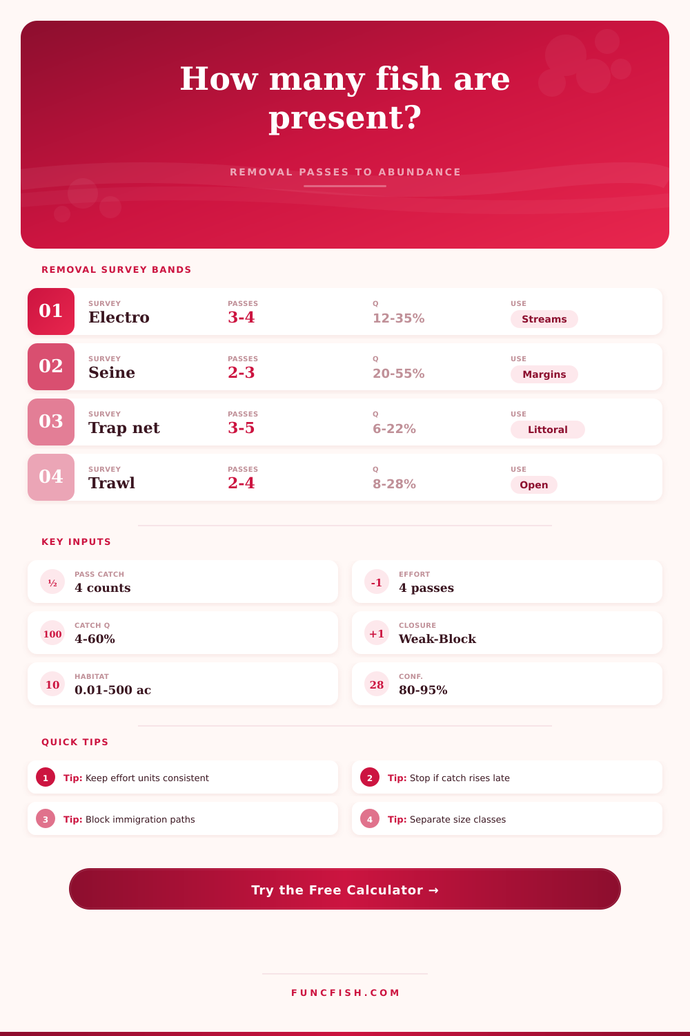
| Backpack electrofishing | 18% to 45% | Blocked wadable reaches | Undercut banks can hide fish |
| Boat electrofishing | 10% to 32% | Shoreline coves and arms | Depth and conductivity shift q |
| Seine removal | 25% to 60% | Smooth margins or block nets | Snags reduce sweep efficiency |
| Trap or hoop net | 5% to 20% | Repeated short soak removals | Bait response may change |
| Species group | Behavior signal | Depletion fit | Density cue |
|---|---|---|---|
| Trout and char | Reach-bound, cover-linked | Often strong with blocks | Report by stream reach area |
| Black bass | Cover-oriented shoreline use | Moderate in coves | Separate adult size classes |
| Panfish | Aggregated schools | Strong only in sealed margins | Use several blocked cells |
| Catfish or carp | Patchy and gear-responsive | Often broad intervals | Use as planning abundance |
| Closure strength | Field condition | Model weight | Range effect |
|---|---|---|---|
| Weak | No blocks, longer survey | 45% depletion curve | Wide interval |
| Moderate | Short window, defined bank | 65% depletion curve | Normal interval |
| Strong | Clear barriers or isolated cove | 82% depletion curve | Narrower interval |
| Blocked | Nets, stop logs, or barriers | 94% depletion curve | Tightest interval |
💡Survey checks
Tip: Keep effort units identical across passes. If one pass is a longer shock time or larger seine pull, enter that effort so CPUE depletion is not overstated.
Tip: Treat late catch increases as a closure warning. Movement into the site, schooling, or changed gear efficiency can make a removal estimate look too small.
Measuring fish gives you look into a world you couldn’t otherwise see. The water looks empty from your position on the shore of a lake or stream, but there’s life below.
There are lots of ways to do this, but the goal isn’t just to know how many fish there is; it’s to figure out how many you have accounted for by the end of survey. With depletion sampling, we treat habitat as a closed system temporarily. We take a few fish out, then we take some more out and observe the catch rate decline. If there is plenty of population, the catch remains strong. If there isn’t much population, the catch will rapidly diminish. It’s simple math, but it’s in the fieldwork that estimates goes awry.
How to Count Fish Accurately
So the first thing you do is set correct boundary. If they are escaping to deeper water or swimming in from upstream as you work, you can’t get a good idea of how many is there. That’s where strength of the closure comes into play. Strong closure would be backpack electrofishing inside of a wadable reach with block nets at each end. Population essentially is sealed. Weak closure occurs when using boat electrofishing in an open arm of a lake. In this case, fish will escape the shock or move in and out with current. The calculator assumes this and will adjust weight accordingly. When the system is blocked it relies more on the depletion curve; but when the system is open, it moves towards catchability coefficients. It’s a subtle shift in the model but makes a big difference in the confidence interval.
The other variable error source is catchability, which is defined as percent of fish caught for every unit of effort used. Catchability vary by species, gear, and water conditions. It’s not natural law. For example, seine nets have very high catchability (sometimes over 60% in shallow margins), sweeping aggressively. Trap nets has low catchability (five to twenty percent) and tend to be selective and slow. This is why you must use a realistic catchability based off your own local calibration (from literature or other sources). Guessing too high will underestimate population size. Guessing too low will inflate the population size. These variables is blended together into an assessment of most probable abundance.
Make each pass take same amount of effort. To get a clean signal about depletion, all your passes should takes the same amount of effort. If it took you an hour to complete the first pass but only took twenty minutes for the second, the depletion signal will be muddy because it’ll also reflect the different amount of time spent in the water. Match the effort so that decrease in catch actually reflects a decrease in population.
The raw data for catch and effort by pass are found here. Look at the pattern. If there’s a steep decline in catch per unit effort between pass one and pass four, then that’s a good thing. That indicates the model is functioning. If the catch remains flat or increases, something isn’t right. Gear efficiency may have changed, or perhaps fish were schooling, which would make them easier to catch. The tables on the page (reference) can help you understand these signals.
The second factor is species behavior. Trout will suspend in cover and remain stationary. When they are blocked in an area, they are depleted in a predictable way. On the other hand panfish are more prone to move around and to school. The tool accounts for this tendency of groups by modifying variation that goes into the end estimate.
The tool doesn’t give you just one number but a range. This range is honest because it recognizes the uncertainty in any biological survey. Don’t overlook the later passes. These are the bottom end of the population and may be its defining characteristic. Stopping on pass 2 means you risk missing the right-hand side of distribution. Pass 4 is the tie-breaker; it tells the difference between a large, robust population and a small, easily exhausted one.
If you’re not sure where to begin, try the presets. There are simple settings for typical situations such as an electrofishing survey of bass out of a boat, or brook trout in a block-net run. But always examine the assumptions. How do you define your system? That’s the key to abundance estimation. Your estimate is only as accurate as your definition of the system.
It’s not that you’re just counting fish. What you’re doing is estimating how many you might be able to see based on what you know about yourself. And then you extend that estimate to the rest of the system. It’s also understanding that the snapshot you take with the final number will never truly represent the whole story. Because the system is in flux; dynamic. For a brief instant you’ve managed to freeze time enough to understand it.
Keep things clear by defining your terms well. Keep your effort constant. Keep your catchability realistic. Everything else is simply math.