Insect Drift Density Calculator
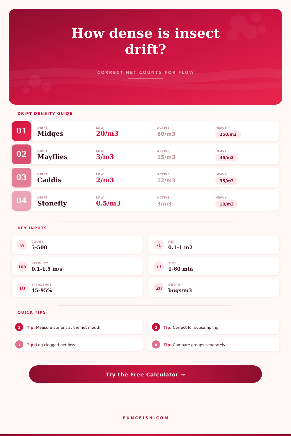
Convert drift-net insect counts into corrected bugs per cubic meter, lane flux, sampled water volume, and feeding signal using net area, current speed, soak time, subsampling, and capture loss.
📌Drift presets
⚙Sample inputs
Density is corrected count divided by sampled volume. Use velocity at the net mouth, not a far-bank current estimate, because small errors compound quickly.
Insect drift estimate
Formula breakdown
📋Drift correction grid
Net opening
Velocity
Efficiency
Drift class
📊Reference tables
| Insect group | Low drift | Active drift | Heavy drift | Typical size |
|---|---|---|---|---|
| Midges / chironomids | Below 20/m³ | 20-120/m³ | 120+/m³ | 2-6 mm |
| Mayfly nymphs | Below 3/m³ | 3-25/m³ | 25+/m³ | 5-14 mm |
| Baetis / small olives | Below 5/m³ | 5-40/m³ | 40+/m³ | 4-8 mm |
| Caddis pupae or larvae | Below 2/m³ | 2-18/m³ | 18+/m³ | 6-16 mm |
| Stonefly nymphs | Below 0.5/m³ | 0.5-5/m³ | 5+/m³ | 12-35 mm |
| Large stonefly / salmonfly | Below 0.2/m³ | 0.2-2/m³ | 2+/m³ | 25-50 mm |
| Terrestrial insects | Below 1/m³ | 1-10/m³ | 10+/m³ | 4-18 mm |
| Hellgrammites / dobsonfly larvae | Below 0.1/m³ | 0.1-1/m³ | 1+/m³ | 30-70 mm |
| Sampling method | Base efficiency | Best use | Common bias | Correction cue |
|---|---|---|---|---|
| Standard drift net | 78% | Mixed nymph drift | Moderate fine loss | Use measured current |
| Fine mesh larval net | 88% | Midges and small baetis | Clogs faster | Raise retention loss |
| Coarse field screen | 62% | Large nymph checks | Small insects pass through | Do not compare to fine mesh |
| Surface film net | 70% | Emergers and terrestrials | Misses near-bed drift | Class as surface signal |
| Near-bed frame net | 74% | Stoneflies and caddis | Bed contact changes flow | Watch mouth blockage |
| Boat-held current net | 68% | Broad river transects | Boat speed error | Average multiple passes |
| Water context | Lane factor | Drift timing | Fish response | Field note |
|---|---|---|---|---|
| Gravel riffle | 1.08 | Day and evening pulses | Fast trout lanes | Sample at riffle tail |
| Steady trout run | 1.00 | Consistent mixed drift | Balanced feeding lane | Good comparison reach |
| Stable tailwater | 0.92 | Long midge windows | Selective feeding | Fine mesh helps |
| Spring creek glide | 0.86 | Small insect pulses | Slow clear-water takes | Avoid weed debris |
| Freestone pocket water | 1.16 | Weather and flow spikes | Opportunistic feeding | Repeat after level changes |
| Undercut bank edge | 1.22 | Wind and shade drops | Terrestrial focus | Separate surface samples |
| Lake or pond inlet | 0.74 | Concentrated inlet plume | Panfish and trout stack | Sample plume centerline |
| Night drift window | 1.34 | After-dark invertebrate movement | Large prey confidence | Use light consistently |
| Fish target | Preferred drift | Useful density cue | Flux cue | Presentation match |
|---|---|---|---|---|
| Trout | Mayfly, midge, caddis | Active or heavy group band | 30+ bugs/m²/min | Match size and drift lane |
| Grayling | Midge and small mayfly | Moderate small-insect density | 20+ bugs/m²/min | Fine tippet and small fly |
| Panfish | Midge, terrestrial, caddis | Dense inlet or bank pulse | 25+ bugs/m²/min | Small float or micro jig |
| Smallmouth bass | Hellgrammite, stonefly, caddis | Large insect signal matters | 5+ large bugs/m²/min | Tube, nymph, or soft plastic |
| Juvenile salmonids | Midge and baetis | Stable small prey density | 15+ bugs/m²/min | Small suspended pattern |
| Carp or suckers | Caddis, midge, mayfly | Bottom-oriented drift pulse | 10+ bugs/m²/min | Nymph close to bottom |
🧭Insect comparison grid
| Insect type | Drift behavior | Best sample window | Count risk | Fishery meaning |
|---|---|---|---|---|
| Midges / chironomids | Steady tiny drift | Cold mornings and tailwaters | Under-counted by coarse mesh | Strong small-fly signal |
| Mayfly nymphs | Pulsed pre-emergence drift | Late morning to evening | Mixed with spent shucks | Classic trout feeding cue |
| Caddis pupae or larvae | Evening and dislodged drift | Warm riffle edges | Cases skew volume | Useful swing or nymph cue |
| Stonefly nymphs | Low-count high-value drift | Night and high flow edges | Easy to miss in short samples | Large prey opportunity |
| Terrestrial insects | Surface and bank-driven drop | Windy shaded banks | Surface nets only see part | Bank-feeding confidence |
| Hellgrammites | Rare dislodged bottom drift | Rocky runs after flow change | Counts are naturally sparse | Large bass and trout cue |
💡Practical checks
Tip: If the net clogs with algae or leaves, raise retention loss or shorten the soak time. Volume keeps increasing on paper even when the mouth is partly blocked.
Tip: When you split a sample tray, enter the processed share. Counting one quarter of the jar needs a 25% subsample setting before density is comparable.
When the fish rise, anglers believe there should be lots of bugs on the water. The truth is typicaly the reverse. A trout may look like it is gorging itself, but it can actualy eat only one insect every half-minute. Because feeding happen so rarely and at steady intervals, it looks like the fish are having a feast. Knowing about drift density help you interpret the water by distinguishing between actual abundance and the illusion of activity.
It’s not that you’re fishing for the spots with the greatest number of bugs. You’re fishing the ones with just enough bug to stimulate a feeding response without overloading the predator.
How to Count Bugs for Better Fishing
With a simple click, the calculator above figure out the numbers when you plug-in current speed and the dimensions of your nets. But there’s one important variable that many angler neglect: the speed of water near the net mouth. Because we all estimate the velocity based off a twig bobbing on surface, it’s worthless; the drift layer where all those insect are swimming is usually not moving at the same speed as top.
Guessing the velocity wrong will ruin everything about your density estimate. A tiny discrepancy in velocity get magnified to an enormous difference in volume. What seems like a heavy drift might appear sparse, or what looks like a sparse drift might appeared heavy.
Also bear in mind: Drift nets aren’t vacuum cleaners. Clogged with gunk? Efficiency of capture will be lower. Blocked with stuff like algae? Your count go down, because your net isn’t letting any water through. You should of adjust for this loss of retention, so that you don’t underestimate the amount of food present.
This is particularly important if you’re using a fine-mesh net and sampling midge. These insects can be so tiny that they falls through coarser mesh or get lost in the muck. The tool then comes back with the correct density of insect in that sample. From there it produce a lane flux number representing the number of insect passing through a given square meter every minute.
That’s the real-world number we care about when choosing flies. Low flux means fish probably has their noses buried into some kind of structure and wait until something swims by close enough to grab it. High flux means they’re probably feeding heavily, but selectively… Anything that doesn’t fit the current profile (both in terms of species and size) get ignored.
The reference table is on the page because trout really like heavy or active bands of drift, while panfish might completely ignore that same concentration. For example, imagine there are both mayflies and stoneflies drifting. Do their method differ? Yes. Mayfly nymphs pulse-drift. They provide brief, concentrated periods followed by nothingness, which triggers frenzied feeding. While stonefly nymphs do not pulse-drift much, if at all, each represent a high-value meal, requiring an accurate presentation.
So while it’s true that a high-density midge might yield fewer bites than a lower density stonefly, if you show them the appropriate pattern with the correct depth, it could of being more. Knowing how often the offering appears (the density number) gives us information, but what we see on the water help us understand its value (offer).
These numbers change over seasons as well. On a spring creek glide, with its slow water and crystal clarity, the Lane Factor tend to be low (making them skittish). On a post-storm freestone river, where the insect-purging flow wash bugs off the bottom and the commotion hide your presence from them, the Lane Factors is likely high. Knowing how these variables affect the numbers will let you know whether what you see is feast or famine; ten insects per cubic meter may be a banquet in a calm tailwater, but a famine in a roiling freestone run.
This is the bottom line. So again, you’re not fishing for data here. You’re fishing for the right combination of timing and pattern to match the fish’s appetite against how much food is drifting by.
So when you get that rise, glance down at the water column and ask yourself… Is this a common bug or is it rare? Does my presentation match what I see happening in the water?
The math takes out the guesswork. The art is what you do with the answer.