Sonar Ping Rate to Depth Calculator
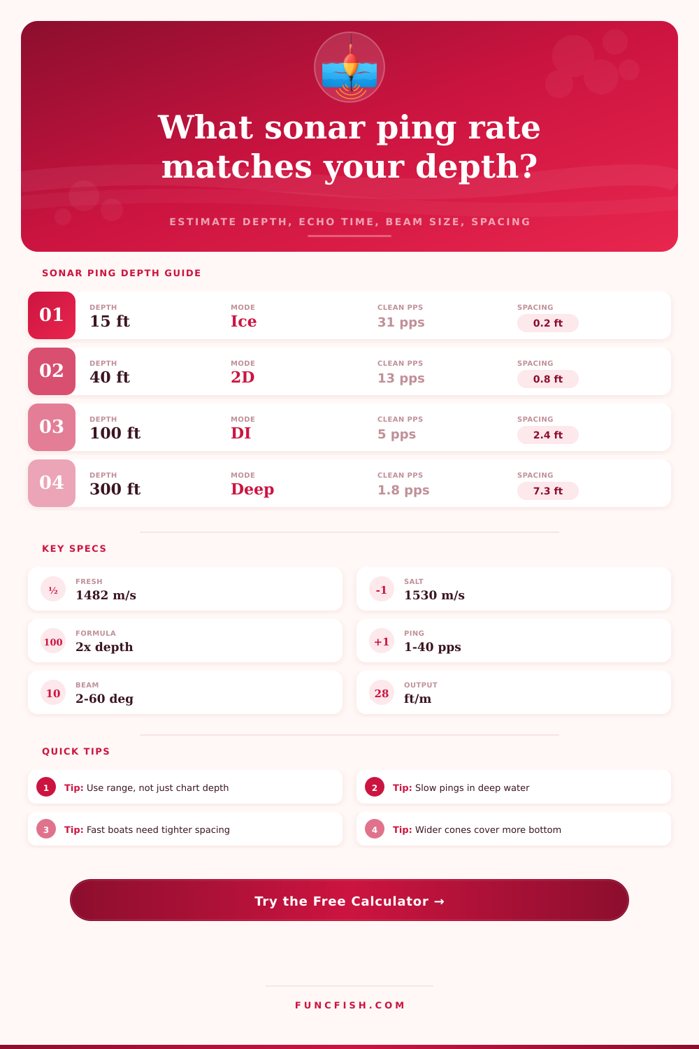
Convert fishing sonar ping rate into clean depth range, echo travel time, bottom footprint, and boat spacing so your graph is matched to the water you are actually scanning.
📌Fishing sonar presets
⚙Ping and depth inputs
Sonar ping result
Formula breakdown
📡Sonar mode data grid
Broad cone for searching shallow cover, bait clouds, and fish off to the sides.
Sharper bottom separation for jigging, dropshots, and fish tight to structure.
Thin scan slices favor detail, but deep ranges demand slower clean updates.
Shorter range and active aiming usually allow faster updates around targets.
🐟Gear and species comparison grid
Short vertical range, tight cone, and nearly zero boat movement make fast pings useful.
Good for 10-50 ft ledges, grass edges, docks, and brush piles with 2D or down imaging.
Balances jig detail and clean bottom reads across 25-80 ft contour passes.
Works around suspended bait and thermoclines where depth range is often expanded.
Moderate deep structure needs slower returns to avoid second-echo confusion.
Spacing matters more than vertical cone size when mapping flats and channels.
Deep bait schools and fast hull speeds require conservative listening windows.
Very deep ranges need long intervals because each echo travels down and back.
📊Reference tables
| Depth range | Round-trip echo time | Balanced max ping rate | Common fishing use |
|---|---|---|---|
| 10 ft / 3.0 m | 4.1 ms at 1482 m/s with 1.15x range | 31-38 pps | Ice holes, docks, shallow grass, kayak sight-fishing lanes |
| 30 ft / 9.1 m | 14.2 ms with reserve and range buffer | 16-22 pps | Bass edges, panfish basins, shallow reefs, bridge pilings |
| 60 ft / 18.3 m | 28.4 ms with reserve and range buffer | 8-13 pps | Walleye breaks, trout trolling, main-lake humps |
| 120 ft / 36.6 m | 56.8 ms with reserve and range buffer | 4-7 pps | Salmon shelves, snapper rubble, deeper bait schools |
| 300 ft / 91.4 m | 142 ms with reserve and range buffer | 1.6-3 pps | Offshore structure, deep rock, suspended tuna forage |
| 900 ft / 274 m | 426 ms with reserve and range buffer | 0.5-1.1 pps | Deep drop, canyon drift, swordfish daytime depth work |
| Sonar mode | Typical beam or slice | Timing allowance | Best calculation use |
|---|---|---|---|
| Wide 2D CHIRP | 35-60 degrees | 2.5 ms blanking, medium pulse | Search coverage and fish arches in shallow to mid-depth water |
| Narrow 2D CHIRP | 12-24 degrees | 2.0 ms blanking, short pulse | Vertical jigging, drop-shotting, and bottom separation |
| Down imaging | 4-12 degrees | 3.2 ms blanking, short pulse | Structure detail directly below the transducer |
| Side imaging | 1.5-4 degrees vertical | 4.5 ms blanking, thin slice | Search passes where along-track spacing controls picture quality |
| Live forward sonar | 12-25 degrees | 2.8 ms blanking, active scan pulse | Aimed casts, fish tracking, and short-range target movement |
| Deep low CHIRP | 10-22 degrees | 5.5 ms blanking, longer pulse | Deep structure, pelagic marks, and long listening windows |
| Water condition | Sound speed used | Effect on depth math | Fishing context |
|---|---|---|---|
| Cold freshwater | 1435 m/s | Slower sound increases travel time and lowers clean ping ceiling | Late fall lakes, winter rivers, ice season edges |
| Temperate freshwater | 1482 m/s | Standard baseline for many inland sonar estimates | Bass, walleye, trout, panfish, and reservoir fishing |
| Warm freshwater | 1495 m/s | Slightly faster returns allow a small ping-rate increase | Summer shallow lakes, ponds, and warm reservoirs |
| Brackish estuary | 1505 m/s | Salt content raises speed compared with freshwater | Striper, redfish, flounder, and tidal river work |
| Cool seawater | 1522 m/s | Faster than freshwater, but deep range still dominates timing | Kelp edges, cold reefs, nearshore rockfish |
| Warm seawater | 1530 m/s | Common marine value for coastal sonar calculations | Snapper, grouper, bait schools, and bluewater marks |
| Tropical saltwater | 1542 m/s | Fastest preset, useful for warm offshore conditions | Pelagics, reefs, and canyon fishing in warm water |
| Boat speed | 5 pps spacing | 10 pps spacing | Use on the water |
|---|---|---|---|
| 0 mph / 0 km/h | 0 ft per ping | 0 ft per ping | Hovering, spot-lock, ice fishing, or vertical jigging |
| 1 mph / 1.6 km/h | 0.29 ft per ping | 0.15 ft per ping | Slow kayak pass, creeping along a weed edge |
| 2.5 mph / 4.0 km/h | 0.73 ft per ping | 0.37 ft per ping | Typical graphing pass for bass, walleye, or crappie |
| 4 mph / 6.4 km/h | 1.17 ft per ping | 0.59 ft per ping | Side imaging search speed over flats and channels |
| 7 mph / 11.3 km/h | 2.05 ft per ping | 1.03 ft per ping | Trolling contour, suspended bait, or salmon water |
| 12 mph / 19.3 km/h | 3.52 ft per ping | 1.76 ft per ping | Fast search pass where screen detail drops quickly |
💡Calculation tips
The sonar isn’t dialed into the sound physics and now there’s nothing but empty water on the screen while the fish sits on your hook. So what? Well, it happened because you relied on equipment without knowing its insides: what pulse it sends out and how it receives those returns. Most of the time, it is simply a matter of timing. Your fancy new transducer might be capable of seeing little fish hiding behind the rock, but it fires down and then just waits for that echo to come back. That wait time are the bottleneck in the data flow. If you fire off another ping before the last one has traveled far enough to avoid hitting the next signal, the result is blanks, ghosts, and overlapped marks.
So we put that into equation by entering our boat speed and depth and the calculator on the page does the rest for us. So you don’t have to guess anymore if what you’re seeing is even physically possible. In slow conditions most guys just crank up the ping rate until they see a smooth image, then they speed up or fish deeper and the image goes to noise. The thing to remember is that sound travels fast in water but it doesn’t happen instantaneously. In fact, it travels about 1482 meters per second in fresh water and a little more quickly in saltwater based off density. But that’s not as important than how far the sound has to travel. If you send a ping out into three hundred feet of water, the sound have to travel six hundred feet total before it gets back to the screen and provides a clean picture.
How to Fix Your Sonar Screen
So how do we make these adjustments? What do they mean? When you dial down ping speed or distance, you’re adjusting how much listening time you have between pings. This accounts for longest possible echo returning before it is overridden by another ping’s return. This is why it factors in the range overhead and then reserves a buffer from that number too. For example, if you set your screen depth to one hundred fifty feet and the bottom is only eighty feet away, it will still listen for the entire length of its window. How could it possibly know the object is shallow unless it hear it echo back? So even in shallow water, your maximum rate of clean ping drops considerably.
When folks complain about their unit not sounding good, it’s not because of signal processing or transducer frequency as much as lack of spacing between transmissions. Another wrinkle is beam width, and it’s dependent upon how you fish. A wider beam creates a bigger footprint on the bottom. This smears the detail over a larger area of the lake bed, but the cone is also wider and covers more ground. Narrower beams has greater definition right below the boat, but when fishing quickly they fail to “see” what’s out to the side. How far does the boat travel from ping to ping are crucial as well, especially while trolling or side scanning quickly. No matter how sensitive the receiver is, if you’re travelling 10 feet with every pulse there will be holes in your presentation. Slower is better but slowing the ping rate down makes sure each shot paints a full portrait before launching into the next.
But here’s the thing: Your need for a smooth screen doesn’t matter to the physics governing sound reflection. Data integrity conflicts with update speed. If you want fast updates, accept lower data integrity. On the other hand, if you want clear images, slow down your pings. At depths of less than twenty feet in shallow water, you can be more aggressive with ping rates as the echo comes back almost instantly. As depth grows, so must listening window, which gets longer and longer exponentially. What felt frantic at ten feet might seem sluggish at two-hundred, but that’s what’s needed for clarity.
The chart on the page matches common fishing situations against their respective safe operating limits. The problem is most folks mess around far more with sensitivity and gain than they do manage the transmit rate. Ping rate is how fast you are sending a pulse out and gain is volume. The more you turn up the gain on an echo rich signal, the louder the overlapping signals become, just amplified. Making that messy looking graph louder will not make it cleaner. You need to leave the system some room to breathe.
Your anchor should of be your depth setting. Ask the calculator for the maximum theoretical rate for clean returns in these conditions. Dial back a bit to compensate for possible temperature changes or plants that scatter sound waves randomaly. Patience can be the difference between seeing fish on top of a grass flat and looking at nothing but empty space.
We love fast updates. It feels like we are watching a live video of what’s going on below. But sonar isn’t video. It’s a chain of snapshots connected through both distance and time. Allow for the travel time and the bottom will open up. If the boat is moving quickly or the water depth is greater, slow the ping rate down. Let it finish its sentence and trust the physics instead of thinking you know how the screen ought to look. Eventually your graph will show the truth if you let it finish displaying data before you ask for something else.